

Comparing Apples to Oranges
Aug 15, 2021Using cosine theta as a statistical similarity metric for comparing chemical fingerprints.
What coding language is best?
Often when talking to data scientists you come to realise that the industry is full of more cliques than classic high-school comedy ‘Mean Girls’. The R & Python users are the Robbin hoods of the industry, boasting that everything should be open source. Great merit towards this but comes with the caveat that you need to have all the free time in the world to bang your head against the wall solving your own bugs. The MATLAB users are typically from academia and boast about formal coding education. While as great as it is, MATLAB requires the user to dip into their grant money and splurge on the MATLAB user interface. From my experience even as a person who dabbles in MATLAB, the experience really gives me PTSD of old Windows XP user interfaces. However, from my recollection of graduate school Windows XP operating systems are still kicking around in some labs. Then there comes the few that see time saving as a return on investment and opt for niche statistical packages coming from companies such as SAS. Although a user in all these platforms, I fall in the later category the most. Sometimes, I don’t want to import libraries such as ‘tidyverse’ for simple data manipulation and enjoy the user interface that SAS incorporates through their JMP software. As much as time saver JMP is it lacks an important characteristic that R & Python excel at; simple matrix calculations and user defined functions aren’t accessible. I know right, why use this software? Well, the data interactivity side of JMP more than makes up for the lack of these operations. The way JMP has solved the issue of not having these functions is having an integration with open-source languages such as R & Python. Okay enough of the opinion piece, let’s get down to showcasing the project using this integration.
Project: Comparing apples to oranges. Using cosine theta as a statistical similarity metric for comparing chemical fingerprints.
My graduate supervisor had this saying that he religiously told me, “In science, every question is essentially the same question”. To this day I constantly hear his voice repeating this when I’m throw into a new project. Whether I’m wearing the hat of a forensic toxicologist or analytical chemist or environmental forensics specialist, I get tasked with the same question: “Are these measured sample the same or different?”. Essentially, my job is to compare the chemical fingerprints or profiles and showcase justifications on to why they are the same or different. What the veterans of my industry used to do before was take a print off of the chromatograph for that sample (chemical analyzer result) and tape samples side be side on their office walls. After staring for a long period of time, their eyes would adjust, and they could see what peaks are elevated or missing. Then based on the similarities or differences they would state the samples came from the same chemical mixture (same source). Then came Excel and consultants could use specific measurements from the instrument and construct chemical profiles. I won’t begin ranting about my opinion on the use of Excel as a tool for data science. In short, yes you can construct a chemical profile in the form of a bar graph, yes you can stare at this for hours (as I did early on in my education) but are you really listening to your data or are you making a subjective opinion based on what you and you alone notice. However, not all scientists fall into this pitfall. As you can tell from my last blog, sometimes the stuff from our grade school trigonometry classes can be the fundamentals used in your machine learning algorithms. For comparing chemical profiles, the best way to quantitatively compare and provide a similarity metric stems from using cosine theta (cos-Ɵ) values.
What is a (cos-Ɵ) Metric?
In forensic applications, a cosine theta (cos-Ɵ) similarity metric that can be used to compare two histograms by treating each isomer distribution as a multi-dimensional vector, and to calculate the cosine of the angle (Ɵ) between the two vectors. As this metric is comparing the angle between two vectors, magnitude differences between samples does not affect the comparison between species fingerprints in comparison to the previous chemometric techniques (PCA and HCA), which are driven by parametric changes in concentration. For each multivariate sample, where the number of variables (isomers) is equal to n, the species fingerprint may be thought of as an n-dimensional vector. The angle between two sample vectors is a function of the similarity in the two isomer fingerprints. If the two samples are identical, the vectors will be coincident, the angle between the vectors will be 0 degrees, and the cosine of that angle is 1.0. Similarity, if two samples share no common isomeric distributions, the angle defined between them is 90 degrees and the cosine of that angle is zero. Thus, cos-Ɵ is bound between zero and one where zero is indicative of 0 percent vector similarity and 1 is indicative of 100 percent vector similarity. When comparing two samples (samples i and j) with reported concentrations of n chemicals measured in each sample, cos-Ɵ is calculated as follows:

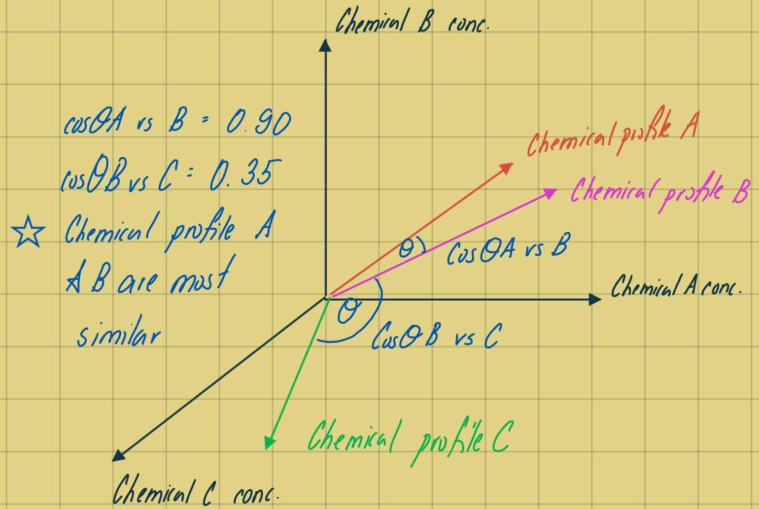
Figure 1 – Cosine Theta anangle between 3 vectors representative of chemical profiles composed of 3 different chemicals (axis). We can see that the angle between the chemical profile of A and B is most similar in vector space and corresponds to a cosine value closer to 1.
Cosine Theta in R
Here I’ll lay out the packages within R that you’ll need, the logic, the source code and the data structure. The source code provided below is an example of taking an excel sheet (instrument generated) and how we can compute the cosine theta similarity between it. Analytes will be row wise, while samples will be column wise for the data matrix.
# Title : Cosine Theta Template
# Created by: Mike Dereviankin
# Created on: 2020-08-17
library(lsa)
temp1 <-read.csv("Cosine Template.csv")
temp1[ ,c('Profile')] <- list(NULL) #Remove unwanted columns
temp2 <-as.matrix(temp1)
temp3 <-as.matrix(cosine(temp2)) write.csv(temp3, "Results.csv")
What you get from running this code is going to be a matrix that is n x n, where every cell is the cosine theta similarity for that sample intersection. Let’s say we’re looking at sample 1 (row 1) x sample 2 (column 2). The number within that cell is going to be how similar the chemical profile of 1 is with 2. Conversely, if we’re looking at sample 2 (row 2) x sample 1 (column 1), this is going to be the same value as it’s comparing the same profiles just backwards.
JMP to R Coding
Let’s say that you’re dealing with a dataset that was recorded using SAS such as the NHANES biomonitoring project conducted by the CDC. R won’t be able to take the individual files from the website without some sort of intermediate step. However, simply clicking the link on the site will allow you to open the files within JMP. Now, you’re tasked with comparing the chemical profiles of individuals in NHANES using a quantitative similarity metric. But, JMP doesn’t have the ability to compute these matrix functions or have a cosine similarity package. What JMP does have is the ability to send data into R, run code in R natively and retrieve all the results without leaving the JMP window. There is a bit of boring download and setting up that is involved, but the people at JMP do a great job at describing it. See this link.
JMP Code
/* Name: Cosine Theta Script
Description: This is the foundation script for the addoin to conduct cosine theta similarity metrices using the R package from lsa called cosine.
Author: Mike Dereviankin
Version: v.1.  */

//Reference the data table being used and transpose columns so that the variable names are rows and samples are columns. Change Columns if need be. Will eventually make this into an add in. The label is the first column that contains the sample names. Adjust accordingly.
//initializes the R interfaces
R Init();

//Name data table
dt = Current Data Table();

//Obtain a list of numeric/continuous column names as strings//
colList = dt << Get Column Names( Continuous, String );

//Function to communicate with R: send script & data to R, get results table back.
//send data to R
R Send( dt );

//Run R code
R Submit (
   "
   library(lsa)
   dt #prints dt to the log
   temp1 <- dt
   temp1[ ,c('Sample')] <- list(NULL) #Remove unwanted columns
   temp2 <-as.matrix(temp1)
   temp3 <-as.matrix(cosine(temp2))
   ");

//return data from R
cosine = R Get(temp3);

cosinetable = As Table( cosine );

//change column names to match the original table

For( i = 1, i <= N Items( colList ), i++,

   Column( cosinetable, i ) << Set Name( colList[i])
   );

//terminates the R interfaces
R Term();
What is even cooler about JMP is that now that we have this code, we can develop a JMP add in (insert link). Here, I’ve got the dataset up so that in a click of a button I can press my handy cosine app and tada I get a huge matrix back. Imagine doing calculation by hand for thousands of samples.
In the example below, I take the profiles of thousands of PCDD/F chemical profiles and compare each sample. We’re talking about 1000 x 1000 calculations in the matter of seconds and all with a click of a button!
Okay brace yourselves this is where Mike’s going to go on a little rant. History is important because we can see how we went from a visually subjective comparison based on “expert” opinion, to streamlining the data into profiles into excel into a finally an objective quantitative similarity metric that is explained by the data and the data alone. The amount of time consulting goes down from days (looking at chemical profiles by the human eye), to hours (excel) to fractions of a second (R code with JMP app). From some consultants this can be seen as a negative; billable time goes down from days to seconds. However, that is what separates a mediocre consultant who rejects the idea of improvement from an innovative one that wants to work to produce the best result for the client. If a consultant is locked away in excel manually doing these calculations by hand, they are spending less time trying to understand their data than the one who simply interprets what the cosine theta algorithm is outputting. I heard this great story about Picasso, and I think it really applies to the profession of consulting. A lady recognizes Picasso in the street and goes up to him and asks, “I love your work, would you mind doing a portrait of me”. Having his supplies on him Picasso agrees and sits the women down to paint her. 5 minutes later he completes the painting and hands it to the women. She says, “How much will it be?”. To which Picasso replies, “10,000 euros”. I made that number up, but she replies, “WHAT!? It only took you 5 minutes.” Picasso replies with, “No madam, it took my whole life to learn how to paint”. The same could be said with consulting. We start from learning the fundamentals and streamline along the way.
Always love to talk more about integration of this into your forensic workflow! Feel free to get in contact and we can talk more about quantitatively comparing fingerprin
MAKE YOUR DATA TALK.
Let's explore the ways I can support you.
Stay connected with news and updates!
Join our mailing list to receive the latest news and updates from our team.
Don't worry, your information will not be shared.
We hate SPAM. We will never sell your information, for any reason.
